Collective Communication¶

In Point-to-Point Communication, we encountered a bottle neck in our trapezoidal rule program. It arose because we were requiring one process to sum the results of all the other processes. In the case of the code presented in the previous chapter, the root process 0 did all the work of summing the results while the other processes idled. A more efficient algorithm would balance the work-load so that there are non-idling processes. This problem can be somewhat corrected through what is called “Collective Communication.” Besides helping to alleviate load imbalances, however, collective communication has a more important purpose: it helps to optimize message passing among separate processes. Communication among processes is expensive. Because each message must be sent over some sort of network, we must minimize and optimize this inter-process communication. In this chapter we show how this can be accomplished in-part with collective communication.

Note

There are two important principles to remember here:

Load Balancing: A program is inefficient if it is not using all of the available resources (e.g., processes are idling because they are waiting on another)
Communication is Expensive: Broadcast and Reduce are designed to optimize communication among the whole communicator. However, any sort of message passing is extremely expensive and one of the main obstacles to obtaining speedups when parallelizing an algorithm.

Tree-Structured Computation¶

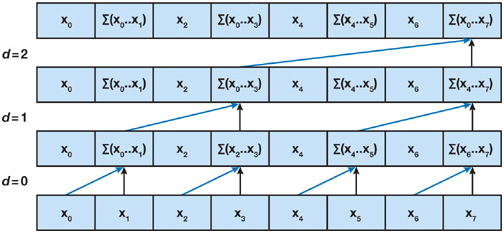
Suppose we have eight processes, each with a number to be summed. Let the even ranked processes send their data to the odd process one greater than each respective process. The odd processes receive data from directly below them in rank. By so doing, we have in one time-step done half of the work.

Fast Summation¶

From this point we can repeat the process with the odd processes, further partitioning them. A summation done in this manner creates a tree structure (see Fast Summation). MPI has implemented fast summations and much more in methods referred to as “Collective Communication.” The method shown in the figure is called Reduce.

Furthermore, MPI has methods that can also distribute information in efficient ways. Imagine reversing the arrows in the figure Fast Summation. This is MPI’s Broadcast function. We should note, though, that the image is a simplification of how MPI performs collective communication. In practice, it is different in every implementation, and is usually more efficient than the simplified example shown. MPI is designed to optimize these methods under the hood, and so we only need to worry about properly applying these functions.

Knowing this, let’s look at the revised trapezoid rule.

The Parallel Trapezoidal Rule 2.0¶

Below is the code for our revised edition of the trapezoid rule. Highlighted in bold is the main change that occurred between the two versions. The statement comm.Reduce(integral, total) has replaced the entire if else statement, including the for loop. Not only does the code look cleaner, it runs faster. The first argument, integral, is the number which is going to be added up, and which is different for every process. The variable total will hold the result:

#trapParallel_2.py
#example to run: mpiexec -n 4 python26 trapParallel_2.py 0.0 1.0 10000
import numpy
import sys
from mpi4py import MPI
from mpi4py.MPI import ANY_SOURCE

comm = MPI.COMM_WORLD
rank = comm.Get_rank()
size = comm.Get_size()

#takes in command-line arguments [a,b,n]
a = float(sys.argv[1])
b = float(sys.argv[2])
n = int(sys.argv[3])

#we arbitrarily define a function to integrate
def f(x):
        return x*x

#this is the serial version of the trapezoidal rule
#parallelization occurs by dividing the range among processes
def integrateRange(a, b, n):
        integral = -(f(a) + f(b))/2.0
        # n+1 endpoints, but n trapazoids
        for x in numpy.linspace(a,b,n+1):
                        integral = integral + f(x)
        integral = integral* (b-a)/n
        return integral


#h is the step size. n is the total number of trapezoids
h = (b-a)/n
#local_n is the number of trapezoids each process will calculate
#note that size must divide n
local_n = n/size

#we calculate the interval that each process handles
#local_a is the starting point and local_b is the endpoint
local_a = a + rank*local_n*h
local_b = local_a + local_n*h

#initializing variables. mpi4py requires that we pass numpy objects.
integral = numpy.zeros(1)
total = numpy.zeros(1)

# perform local computation. Each process integrates its own interval
integral[0] = integrateRange(local_a, local_b, local_n)

# communication
# root node receives results with a collective "reduce"
comm.Reduce(integral, total, op=MPI.SUM, root=0)

# root process prints results
if comm.rank == 0:
        print "With n =", n, "trapezoids, our estimate of the integral from"\
        , a, "to", b, "is", total

The careful observer may have noticed from the figure :ref:fastSum that in the end of the call to Reduce, only the root process holds the final summation. This brings up an important point: collective communication calls can return different values to each process. This can be a “gotcha” if you are not paying attention.

So what can we do if we want to return the same result for a summation to all processes: use the provided subroutine AllReduce. It does the same thing as Reduce, but it simultaneously uses each process as the root. That way, by the end of the summation, each process has calculated an identical sum. Duplicate work was done, but in the end, the result ends up on each process at the same time.

So when should we use Reduce, over AllReduce? If it is unimportant for all processes to have the result, as is the case with the Trapezoidal Rule, using Reduce should be slightly faster than using AllReduce. On the other hand, if every process needs the information, AllReduce is the fastest way to go. We could come up with some other solutions to the situation, such as a call to Reduce, followed by a call to Broadcast, however these other solutions are always less efficient than just using one call to the collective communication routines. In the end, the less communications, the better.

Theoretically, Allreduce could be just as fast as Reduce. Insert Butterfly communication pattern here. TODO

Reduce(…) and Allreduce(…)¶

Comm.Reduce(sendbuf, recvbuf, Op op = MPI.SUM, root = 0)¶

Reduces values on all processes to a single value onto the root process.

Parameters

Comm (MPI comm) – communicator we wish to query
sendbuf (choice) – address of send buffer
recvbuf (choice) – address of receive buffer (only significant at root)
op (handle) – reduce operation
root (int) – rank of root operation

Example:

import numpy
from mpi4py import MPI
comm = MPI.COMM_WORLD

rank = comm.Get_rank()
rankF = numpy.array(float(rank))
total = numpy.zeros(1)
comm.Reduce(rankF,total, op=MPI.MAX)

Comm.Allreduce(sendbuf, recvbuf, Op op = MPI.SUM)¶

Reduces values on all processes to a single value onto all processes.

Parameters

Comm (MPI comm) – communicator we wish to query
sendbuf (choice) – starting address of send buffer
recvbuf (choice) – starting address of receive buffer
op (handle) – operation

Example:

Same as the example for Reduce except replace comm.Reduce with comm.Allreduce. Notice that all process now have the “reduced” value.

Note

Within the Op class are values that represent predefine operations to be used with the “reduce” functions. There are also methods that allow the creation of user-defined operations. I present here a table of the predefined operations. Full documentation is found here: http://mpi4py.scipy.org/docs/apiref/mpi4py.MPI.Op-class.html

The Op Class (Reduction Operators)¶

These are the predefined operations that can be used for the input parameters Op (usage: comm.Reduce(sendbuf,recvbuf, op=MPI.PROD)). For more informaiton, see the section in the appendix, The Op Class (Reduction Operations).

Name	Meaning
MPI.MAX	maximum
MPI.MIN	minimum
MPI.SUM	sum
MPI.PROD	product
MPI.LAND	logical and
MPI.BAND	bit-wise and
MPI.LOR	logical or
MPI.BOR	bit-wise or
MPI.LXOR	logical xor
MPI.BXOR	bit-wise xor
MPI.MAXLOC	max value and location
MPI.MINLOC	min value and location

Dot Product¶

Calculating a dot product is a relatively simple task which does not need to be parallelized, but it makes a good example for introducing the other important collective communication subroutines. When provided two vectors, the dot product, is simply the sum of the element wise multiplications of the two vectors:

\[\sum_{k=1}^{n}u_{k}v_{k}\]

Parallelizing the Dot Product¶

Speedups can be gained by parallelizing the previous operation. We can divide up the work among different processors by sending pieces of the original vectors to different processors. Each processor then multiplies its elements and sums them. Finally, the local sums are summed using Comm.Reduce, which sums numbers distributed among many processes in O(log n) time. The procedure is as follows:

Divide the n-length arrays among p processes.
Run the serial dot product on each process’s local data.
Use Reduce with MPI_SUM to collect the result.

First, we must divide up the array. We will do this with the function Scatter(...). THen, we must write the code that implements the serial operation. For this, we just call numpy’s implementation: numpy.dot(a, b). We conlude with Reduce(...).

The code looks like this:

#dotProductParallel_1.py
#"to run" syntax example: mpiexec -n 4 python26 dotProductParallel_1.py 40000
from mpi4py import MPI
import numpy
import sys

comm = MPI.COMM_WORLD
rank = comm.Get_rank()
size = comm.Get_size()

#read from command line
n = int(sys.argv[1])    #length of vectors

#arbitrary example vectors, generated to be evenly divided by the number of
#processes for convenience

x = numpy.linspace(0,100,n) if comm.rank == 0 else None
y = numpy.linspace(20,300,n) if comm.rank == 0 else None

#initialize as numpy arrays
dot = numpy.array([0.])
local_n = numpy.array([0])

#test for conformability
if rank == 0:
                if (n != y.size):
                                print "vector length mismatch"
                                comm.Abort()

                #currently, our program cannot handle sizes that are not evenly divided by
                #the number of processors
                if(n % size != 0):
                                print "the number of processors must evenly divide n."
                                comm.Abort()

                #length of each process's portion of the original vector
                local_n = numpy.array([n/size])

#communicate local array size to all processes
comm.Bcast(local_n, root=0)

#initialize as numpy arrays
local_x = numpy.zeros(local_n)
local_y = numpy.zeros(local_n)

#divide up vectors
comm.Scatter(x, local_x, root=0)
comm.Scatter(y, local_y, root=0)

#local computation of dot product
local_dot = numpy.array([numpy.dot(local_x, local_y)])

#sum the results of each
comm.Reduce(local_dot, dot, op = MPI.SUM)

if (rank == 0):
                print "The dot product is", dot[0], "computed in parallel"
                print "and", numpy.dot(x,y), "computed serially"

The important parts of this algorithm are the collective communications, highlighted in the source code. The first call, which is to Bcast(...), simply tells the other processors how big of an array to allocate for their portion of the original vectors: they will each allocate n/size slots for x and for y.

The actual distributing of the data occurs with the calls to Scatter(...). Scatter will take an array and divide it up over all the processes. From this point, the serial dot product is run to calculate a local dot product. Now the only thing left to do is to add up the partial sums.

Reduce is the final part of the solution: it is called on line 7, and when it is finished, process 0 will contain the total dot product.

With this new algorithm and enough processors, the runtime approaches O(log n) time. To help understand how much faster this is compared to the original version, imagine that we have as many processors as we have items in each array: say, 1000. Then, each of these operations requires the same amount of time, the algorithm’s runtime would run hypothetically something like this:

Task vs Time	Serial Code	Point-to-Point mpi	Collective mpi
Broadcast n = 1000	N/A	About 1000	About 10
Scatter x	N/A	About 1000	About 10
Scatter y	N/A	About 1000	About 10
Compute sum	1000	1	1
Reduce result	N/A	About 1000	About 10
Total	About 1000	About 4001	About 41

The first column shows the serial dot product’s time requirements. The final column shows the mpi-version. It is clear that the final version requires less time and that this number drops with the number of processors used. We simply cannot get this speed up unless we break out of the serial paradigm.

The middle column illustrates why we should use broadcast, and scatter, and reduce over using n send/recv pairs in a for-loop. We do not include code for this variation. It turns out that using MPI in this fashion can actually run slower than the serial implementation of our dot product program.

Bcast(…) and Scatter(…)¶

Comm.Bcast(buf, root=0)¶

Broadcasts a message from the process with rank “root” to all other processes of the group.

Parameters

Comm (MPI comm) – communicator across which to broadcast
buf (choice) – buffer
root (int) – rank of root operation

Example:

import numpy
from mpi4py import MPI
comm = MPI.COMM_WORLD
rank = comm.Get_rank()

#intialize
rand_num = numpy.zeros(1)

if rank == 0:
        rand_num[0] = numpy.random.uniform(0)

comm.Bcast(rand_num, root = 0)
print "Process", rank, "has the number", rand_num

Comm.Scatter(sendbuf, recvbuf, root)¶

Sends data from one process to all other processes in a communicator (Length of recvbuf must evely divide the length of sendbuf. Otherwise, use Scatterv)

Parameters

sendbuf (choice) – address of send buffer (significant only at root)
recvbuf (choice) – address of receive buffer
root (int) – rank of sending process

Example:

import numpy
from mpi4py import MPI
comm = MPI.COMM_WORLD
rank = comm.Get_rank()
size = comm.Get_size()
LENGTH = 3

#create vector to divide
if rank == 0:
        #the size is determined so that length of recvbuf evenly divides the
        #length of sendbuf
        x = numpy.linspace(1,size*LENGTH,size*LENGTH)
else:
        #all processes must have a value for x
        x = None

#initialize as numpy array
x_local = numpy.zeros(LENGTH)

#all processes must have a value for x. But only the root process
#is relevant. Here, all other processes have x = None.
comm.Scatter(x, x_local, root=0)

#you should notice that only the root process has a value for x that
#is not "None"
print "process", rank, "x:", x
print "process", rank, "x_local:", x_local

Warning

The length of the recvbuf vector must evely divide the sendbuf vector. Otherwise, use Scatterv. (The same principle holds for the function Gather and Gatherv which undoes Scatter and Scatterv. See exercise TODO.

A Closer Look at Broadcast and Reduce¶

Let’s take a closer look at the call to comm.Bcast. Bcast sends data from one process to all others. It uses the same tree-structured communication illustrated in the Figure Fast Summation. It takes for its first argument an array of data, which must exist on all processors. However, what is contained in that array may be insignificant. The second argument tells Bcast which process has the useful information. It then proceeds to overwrite any data in the arrays of all other processes.

Bcast behaves as if it is synchronous. “Synchronous” means that all processes are in synch with each other, as if being controlled by a global clock tick. For example, if all processes make a call to Bcast they will all be guaranteed to be calling the subroutine at basically the same time.

For all practical purposes, you can also think of Reduce as being synchronous. The difference is that Reduce only has one receiving process, and that process is the only process whose data is guaranteed to contain the correct value at completion of the call. To test your understanding of Reduce, suppose we are adding the number one up by calling Comm.Reduce on 100 processes, with the root being process 0. The documentation of Comm.Reduce tells us that the receive buffer of process 0 will contain the number 100. What will be in the receive buffer of process 1?

The answer is we don’t know. The reduce could be implemented in one of several ways, dependent on several factors, and as a result it is non-deterministic. During collective communications such as Reduce, we have no guarantee of what value will be in the intermediate processes’ receive buffer. More importantly, future calculations should never rely on this data except in process root (process 0 in our case).

Scatterv(…) and Gatherv(…)¶

Comm.Scatterv([choice sendbuf, tuple_int sendcounts, tuple_int displacements, MPI_Datatype sendtype, ]choice recvbuf, root=0)¶

Scatter data from one process to all other processes in a group providing different amount of data and displacements at the sending side

Parameters

Comm (MPI comm) – communicator across which to scatter
sendbuf (choice) – buffer
sendcounts (tuple_int) – number of elements to send to each process (one integer for each process)
displacements (tuple_int) – number of elements away from the first element in the array at which to begin the new, segmented array
sendtype (MPI_Datatype) – MPI datatype of the buffer being sent (choice of sendbuf)
recvbuf (choice) – buffer in which to receive the sendbuf
root (int) – process from which to scatter

Example:

# for correct performance, run unbuffered with 3 processes:
# mpiexec -n 3 python26 scratch.py -u
import numpy
from mpi4py import MPI
comm = MPI.COMM_WORLD
rank = comm.Get_rank()

if rank == 0:
        x = numpy.linspace(0,100,11)
else:
        x = None

if rank == 2:
        xlocal = numpy.zeros(9)
else:
        xlocal = numpy.zeros(1)

if rank ==0:
        print "Scatter"
comm.Scatterv([x,(1,1,9),(0,1,2),MPI.DOUBLE],xlocal)
print ("process " + str(rank) + " has " +str(xlocal))

comm.Barrier()
if rank == 0:
        print "Gather"
        xGathered = numpy.zeros(11)
else:
        xGathered = None
comm.Gatherv(xlocal,[xGathered,(1,1,9),(0,1,2),MPI.DOUBLE])
print ("process " + str(rank) + " has " +str(xGathered))

Comm.Gatherv(choice sendbuf, [choice recvbuf, tuple_int sendcounts, tuple_int displacements, MPI_Datatype sendtype, ]root=0)¶

Gather Vector, gather data to one process from all other processes in a group providing different amount of data and displacements at the receiving sides

Parameters

Comm (MPI comm) – communicator across which to scatter
sendbuf (choice) – buffer
recvbuf (choice) – buffer in which to receive the sendbuf
sendcounts (tuple_int) – number of elements to receive from each process (one integer for each process)
displacements (tuple_int) – number of elements away from the first element in the receiving array at which to begin appending the segmented array
sendtype (MPI_Datatype) – MPI datatype of the buffer being sent (choice of sendbuf)
root (int) – process from which to scatter

Example:

See the example for Scatterv().

Exercises¶

What is the difference between Reduce and Allreduce?
Why is Allreduce faster than a Reduce followed by a Bcast?
In our parallel implementation of the calculation of the dot product, “dotProductParallel_1.py”, the number of processes must evenly divide the length of the vectors. Rewrite the code so that it runs regardless of vector length and number of processes (though for convenience, you may assume that the vector length is greater than the number of processes). Remember the principle of load balancing. Use Scatterv() to accomplish this.
Alter your code from the previous exercise so that it calculates the supremum norm(the maximal element) of one of the vectors (choose any one). This will include changing the operator Op in the call to Reduce.
Use Scatter to parallellize the multiplication of a matrix and a vector. There are two ways that this can be accomplished. Both use Scatter to distribute the matrix, but one uses Bcast to distribute the vector and Gather to finish while the other uses Scatter to segment the vector and finishes with Reduce. Outline how each would be done. Discuss which would be more efficient (hint: think about memory usage). Then, write the code for the better one. Generate an arbitrary matrix on the root node. You may assume that the number of processes is equal to the number of rows (columns) of a square matrix. Example code demonstrating scattering a matrix is shown below:
```
from mpi4py import MPI
import numpy
comm = MPI.COMM_WORLD
rank = comm.Get_rank()

A = numpy.array([[1.,2.,3.],[4.,5.,6.],[7.,8.,9.]])
local_a = numpy.zeros(3)
comm.Scatter(A,local_a)
print "process", rank, "has", local_a
```

Collective Communication¶

Tree-Structured Computation¶

The Parallel Trapezoidal Rule 2.0¶

Reduce(…) and Allreduce(…)¶

The Op Class (Reduction Operators)¶

Dot Product¶

Parallelizing the Dot Product¶

Bcast(…) and Scatter(…)¶

A Closer Look at Broadcast and Reduce¶

Scatterv(…) and Gatherv(…)¶

Exercises¶

Table of Contents

Previous topic

Next topic

This Page